ວິທີການປ່ຽນສີແຖວໃນ Excel ໂດຍເງື່ອນໄຂ, ຂຶ້ນກັບເງື່ອນໄຂ

In this article, you’ll learn how to quickly change the background of a row based on a specific value in a spreadsheet. Here are guidelines and various formulas for text and numbers in a document.

Previously, we discussed methods for changing the background color of a cell based on text or a numeric value in it. Recommendations will also be presented here on how to highlight the necessary rows in the latest versions of Excel, based on the contents of one cell. In addition, here you will find examples of formulas that work equally well for all possible cell formats.

How to change the appearance of a row based on a number in a specific cell

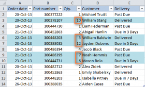
For example, you have a document open with an organization’s deals table like this one.

Suppose you need to highlight rows in different shades, focusing on what is written in a cell in the Qty column, in order to clearly understand which of the transactions are the most profitable. To achieve this result, you need to use the “Conditional Formatting” function. Follow the step by step instructions:

1. ເລືອກຕາລາງທີ່ທ່ານຕ້ອງການຈັດຮູບແບບ.
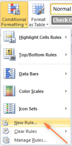
2. Create a new formatting rule by clicking the appropriate item in the context menu that appears after clicking the “Conditional Formatting” button on the “Home” tab.

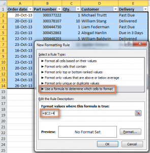
1. After that, a dialog box will appear where you need to select the setting “use a formula to determine formatted cells.” Next, write down the following formula: =$C2>4 ຢູ່ໃນປ່ອງຂ້າງລຸ່ມນີ້. Naturally, you can insert your own cell address and your own text, as well as replace the > sign with < or =. In addition, it is important not to forget to put the $ sign in front of the cell reference in order to fix it when copying. This makes it possible to bind the color of the line to the value of the cell. Otherwise, when copying, the address will “move out”.
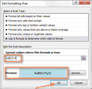
2. Click on “Format” and switch to the last tab to specify the desired shade. If you don’t like the shades suggested by the program, you can always click on “More Colors” and select the shade you need.
3. After completing all the operations, you must double-click on the “OK” button. You can also set other types of formatting (font type or specific cell border style) on other tabs of this window.
4. At the bottom of the window there is a preview panel where you can see what the cell will look like after formatting.
5. If everything suits you, click on the “OK” button to apply the changes. Everything, after performing these actions, all lines in which the cells contain a number greater than 4 will be blue.

As you can see, changing the hue of a row based on the value of a particular cell in it is not the most difficult task. You can also use more complex formulas to be more flexible in using conditional formatting to achieve this goal.

Apply multiple rules according to their priority

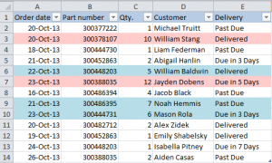
The previous example showed an option to use one conditional formatting rule, but you may want to apply several at once. What to do in such a case? For example, you can add a rule according to which lines with the number 10 or more will be highlighted in pink. Here it is necessary to additionally write down the formula =$C2>9, and then set priorities so that all rules can be applied without conflicting with each other.

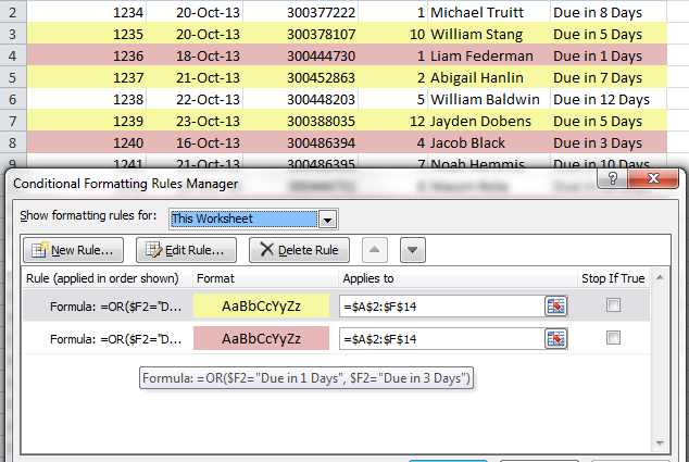
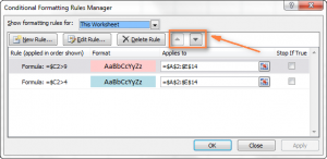
1. On the “Home” tab in the “Styles” group, you need to click on “Conditional Formatting” and in the menu that appears, select “Manage Rules” at the very end of the list.
2. Next, you should display all the rules specific to this document. To do this, you need to find the list at the top “Show formatting rules for”, and select the item “This sheet” there. Also, through this menu, you can configure formatting rules for specific selected cells. In our case, we need to manage the rules for the entire document.
3. Next, you need to select the rule that you want to apply first and move it to the top of the list using the arrows. You will get such a result.
4. After setting the priorities, you need to click on “OK”, and we will see how the corresponding lines have changed their color, according to the priority. First, the program checked to see if the value in the Qty column was greater than 10, and if not, whether it was greater than 4.

Changing the color of an entire line based on the text written in the cell

Assume that while working with a spreadsheet, you have difficulty quickly keeping track of which items have already been delivered and which have not. Or maybe some are out of date. To simplify this task, you can try to select lines based on the text that is in the “Delivery” cell. Suppose we need to set the following rules:

1. If the order is overdue after a few days, the background color of the corresponding line will be orange.
2. If the goods have already been delivered, the corresponding line turns green.
3. If the delivery of goods is overdue, then the corresponding orders must be highlighted in red.

In simple words, the color of the line will change depending on the status of the order.

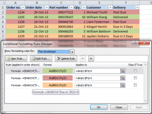
In general, the logic of actions for delivered and overdue orders will be the same as in the example described above. It is necessary to prescribe formulas in the conditional formatting window =$E2=»Delivered» и =$E2=»Past Due» respectively. A little more difficult task for deals that will expire within a few days.

As we can see, the number of days can vary between rows, in which case the above formula cannot be used.

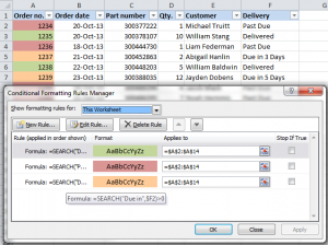
For this case there is a function =SEARCH(“Due in”, $E2)>0, ບ່ອນທີ່:

• the first argument in brackets is the text contained in all described cells,
• and the second argument is the address of the cell whose value you want to navigate.

In the English version it is known as =SEARCH. It is designed to search for cells that partially match the input query.

Tip: The parameter >0 in the formula means that it doesn’t matter where the input query is located in the cell text.

For example, the “Delivery” column might contain the text “Urgent, Due in 6 Hours” and the corresponding cell would still be formatted correctly.

If it is necessary to apply formatting rules to rows where the key cell begins with the desired phrase, then you must write =1 in the formula instead of >0. 

All these rules can be written in the corresponding dialog box, as in the example above. As a result, you get the following:

How to change the color of a cell based on the value in another cell?

Just like with a row, the steps above can be applied to a single cell or range of values. In this example, the formatting is only applied to the cells in the “Order number” column:

How to apply multiple conditions for formatting

If you need to apply several conditional formatting rules to strings, then instead of writing separate rules, you need to create one with formulas =OR or =И. The first means “one of these rules is true,” and the second means “both of these rules are true.”

In our case, we write the following formulas:

=ИЛИ($F2=»Due in 1 Days», $F2=»Due in 3 Days»)

=ИЛИ($F2=»Due in 5 Days», $F2=»Due in 7 Days»)

And the formula =И can be used, for example, in order to check if the number in the Qty column is. greater than or equal to 5 and less than or equal to 10.

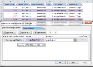
The user can use more than one condition in formulas.

Now you know what you need to do to change the color of a row based on a particular cell, you understand how to set multiple conditions and prioritize them, and how to use multiple formulas at once. Next, you need to show imagination.