ວິທີການເຮັດໃຫ້ຈຸລັງດຽວກັນໃນ Excel

Often when working with Excel spreadsheets, it becomes necessary to edit cell sizes. It is necessary to do this in order to fit all the necessary information there. But because of such changes, the appearance of the table deteriorates significantly. To solve this situation, it is necessary to make each cell the same size as the rest. Now we will learn in detail what actions need to be taken to achieve this goal.

Setting the units of measurement

There are two main parameters related to cells and characterizing their sizes:

1. Column width. By default, values ​​can range from 0 to 255. The default value is 8,43.
2. Line height. Values ​​can range from 0 to 409. The default is 15.

Each point is equal to 0,35 mm.

At the same time, it is possible to edit the units of measurement in which the width and height of the cells will be determined. To do this, follow the instructions:

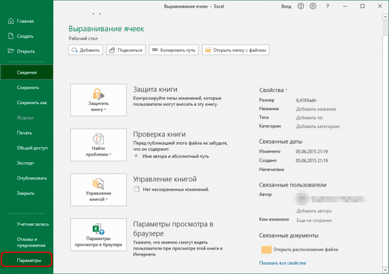
1. Find the “File” menu and open it. There will be an item “Settings”. He must be chosen.
   

   

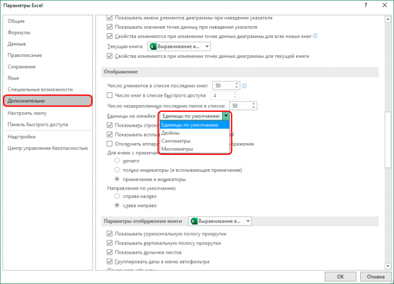
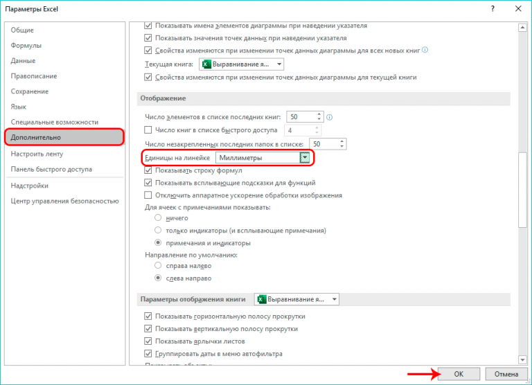
2. Next, a window will appear, on the left side of which a list is provided. You need to find the section “Additionally” and click on it. On the right of this window, we are looking for a group of parameters called "ສະແດງ". In the case of older versions of Excel, it will be called "ຫນ້າຈໍ". There is an option "ຫນ່ວຍງານຢູ່ໃນເສັ້ນ", you need to click on the currently set value to open a list of all available units of measure. Excel supports the following – inches, centimeters, millimeters.
   

   

3. After selecting the desired option, click "ຕົກ​ລົງ".
   

   

So, then you can choose the unit of measurement that is most appropriate in a particular case. Further parameters will be set according to it.

Cell Area Alignment – Method 1

This method allows you to align the cell sizes in the selected range:

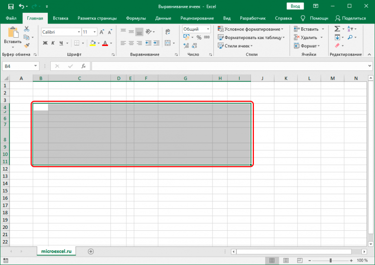
1. Select the range of required cells.
   

   

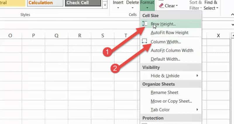
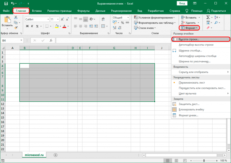
2. ເປີດແຖບ "ບ້ານ"where is the group "ຈຸລັງ". There is a button at the very bottom of it. "ຮູບແບບ". If you click on it, a list will open, where in the very top line there will be an option "ຄວາມສູງຂອງເສັ້ນ". ທ່ານຈໍາເປັນຕ້ອງໃຫ້ຄລິກໃສ່ມັນ.
   

   

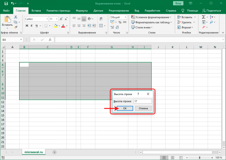
3. Next, a window with timeline height options will appear. Changes will be made to all parameters of the selected area. When everything is done, you need to click on "ຕົກ​ລົງ".
   

   

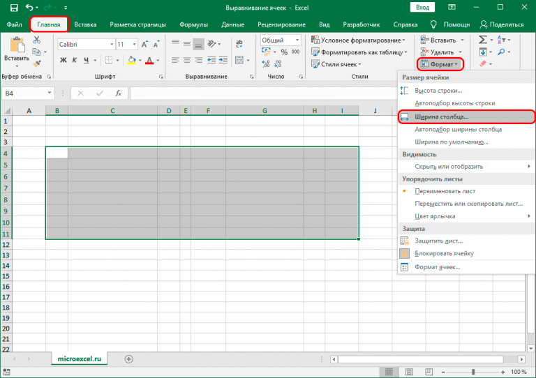
4. After all these actions, it was possible to adjust the height of all cells. But it remains to adjust the width of the columns. To do this, you need to select the same range again (if for some reason the selection was removed) and open the same menu, but now we are interested in the option "ຄວາມກວ້າງຂອງຖັນ". It is third from the top.
   

   

5. Next, set the required value. After that, we confirm our actions by pressing the button "ຕົກ​ລົງ".
   

   

6. Hooray, it’s all done now. After performing the manipulations described above, all cell size parameters are similar throughout the entire range.
   

   

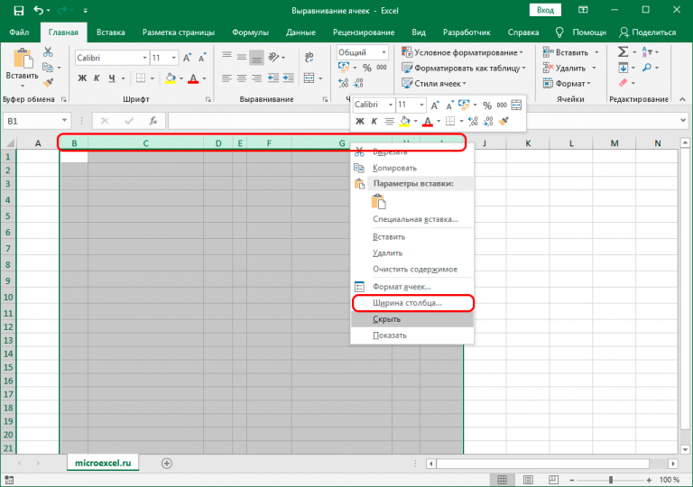
But this is not the only possible method to ensure that all cells have the same size. To do this, you can adjust it on the coordinates panel:

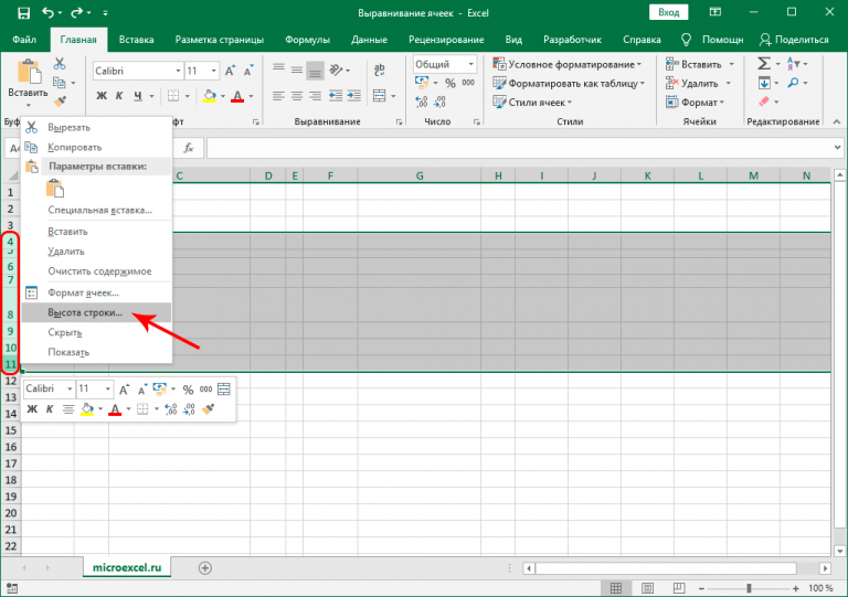
1. To set the required height of the cells, move the cursor to the vertical coordinate panel, where select the numbers of all rows and then call the context menu by right-clicking on any cell of the coordinate panel. There will be an option "ຄວາມສູງຂອງເສັ້ນ", on which you need to click already with the left button.
   

   

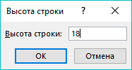
2. Then the same window will pop up as in the previous example. We need to select the appropriate height and click on "ຕົກ​ລົງ".
   

   

3. The width of the columns is set in the same way. To do this, it is necessary to select the required range on the horizontal coordinate panel and then open the context menu, where to select the option "ຄວາມກວ້າງຂອງຖັນ".
   

   

4. Next, specify the desired value and click "ຕົກ​ລົງ".

Aligning the sheet as a whole – method 2

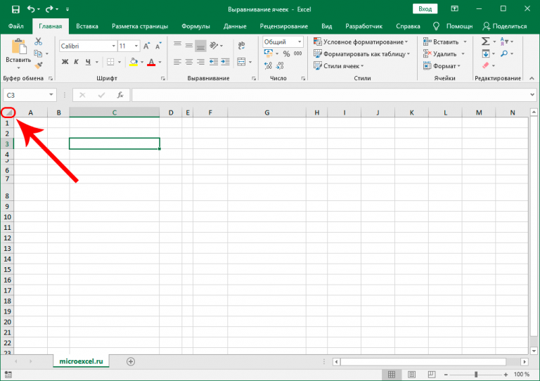
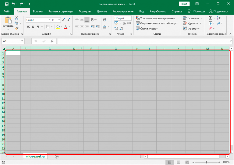
In some cases, it is necessary to align not a specific range, but all elements. 

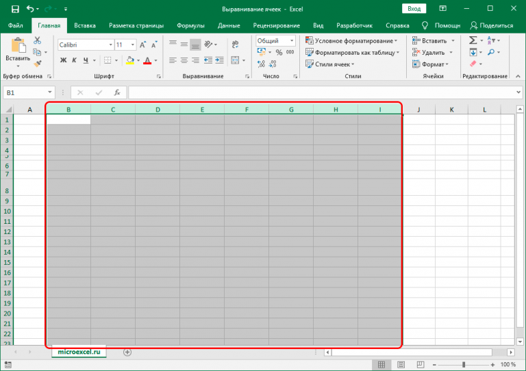
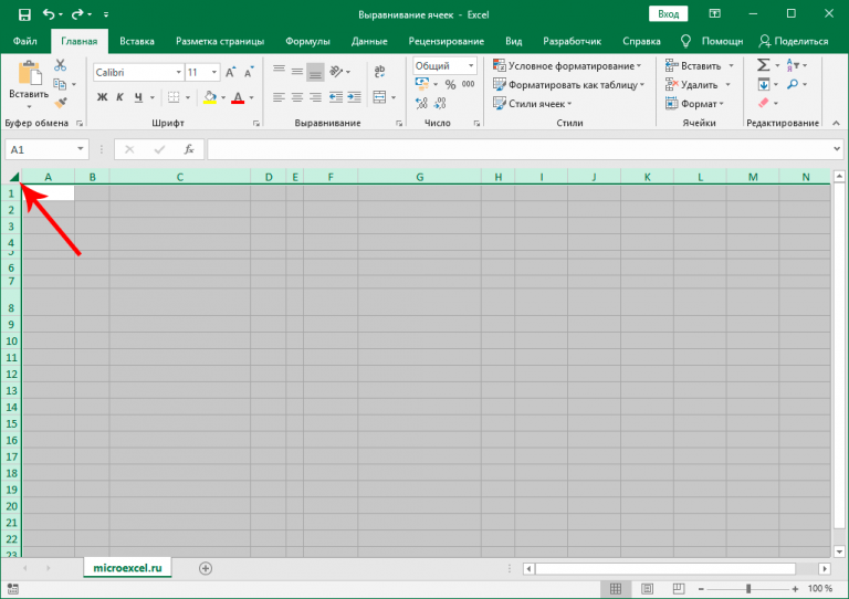
1. Naturally, there is no need for all cells to be selected individually. It is necessary to find a tiny rectangle located at the junction of the vertical and horizontal coordinate bars. Or another option is the keyboard shortcut Ctrl + A.
   

   

2. Here’s how to highlight worksheet cells in one elegant move. Now you can use method 1 to set the cell parameters.
   

   

Self-configuration – method 3

In this case, you need to work with cell borders directly. To implement this method, you need:

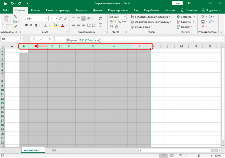
1. Select either a single area or all cells of a specific sheet. After that, we need to move the cursor to any of the column borders within the area that has been selected. Further, the cursor will become a small plus sign with arrows leading in different directions. When this happens, you can use the left mouse button to change the position of the border. Since a separate area was selected in the example we are describing, the changes are applied to it.
   

   

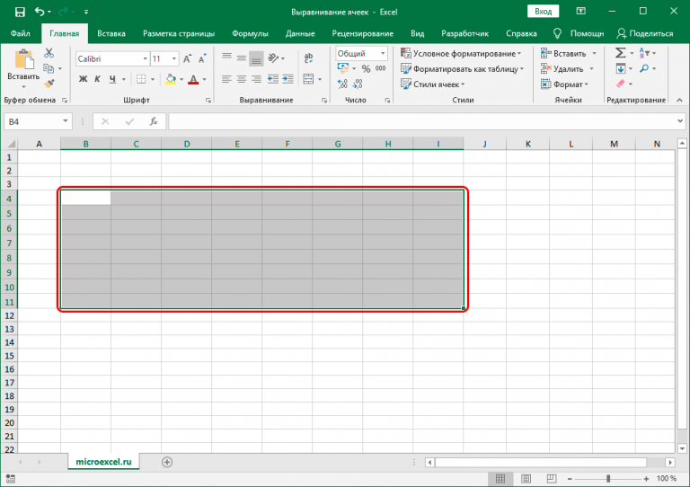
2. That’s it, now all cells in a certain range have the same width. Mission completed, as they say.
   

   

3. But we can see in the screenshot above that the height is still different. To fix this flaw, you need to adjust the size of the lines in exactly the same way. It is necessary to select the corresponding lines on the vertical coordinate panel (or the entire sheet) and change the position of the borders of any of them. 17png
4. Now it’s definitely done. We managed to make sure that all cells are the same size.

This method has one drawback – it is impossible to fine-tune the width and height. But if high accuracy is not necessary, it is much more convenient than the first method.

ສໍາຄັນ! If you want to ensure that all cells of the sheet have the same size, you need to select each of them using a box in the upper left corner or using a combination Ctrl + A, and set the correct values ​​in the same way.

How to align rows after inserting a table – Method 4

It often happens that when a person tries to paste a table from the clipboard, he sees that in the pasted range of cells, their sizes do not match the original ones. That is, the cells of the original and inserted tables have different heights and widths. If you want to match them, you can use the following method:

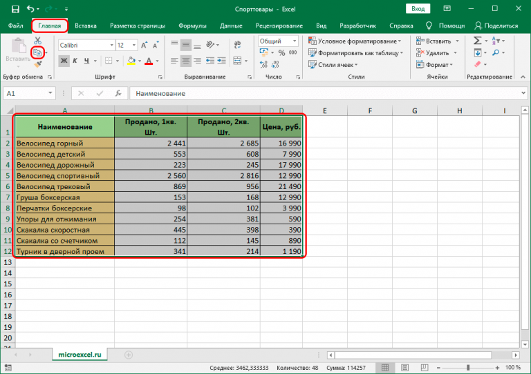
1. First you need to open the table that we need to copy and select it. After that find the tool group "ຄລິບບອດ" ແຖບ "ບ້ານ"where is the button "ສຳ ເນົາ". You have to click on it. In addition, hot keys can be used Ctrl + Cto copy the desired range of cells to the clipboard.
   

   

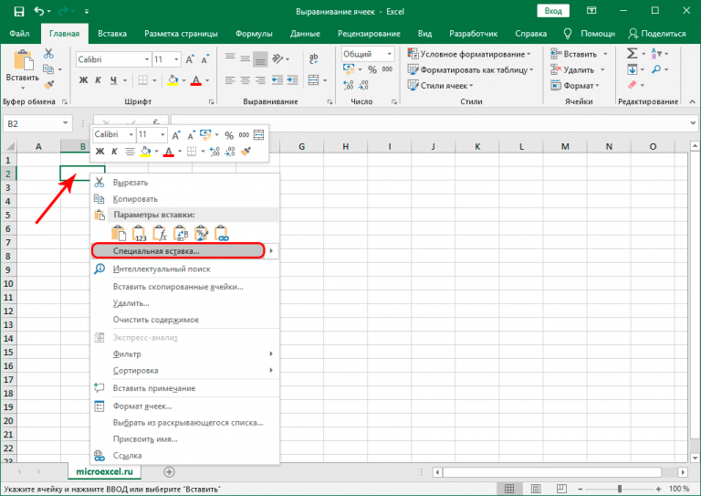
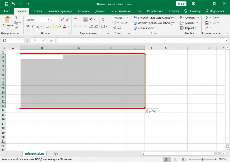
2. Next, you should click on the cell into which the copied fragment will be inserted. It is she who will become the upper left corner of the future table. To insert the desired fragment, you need to right-click on it. In the pop-up menu, you need to find the option “Paste Special”. But do not click on the arrow next to this item, because it will open additional options, and they are not needed at the moment.
   

   

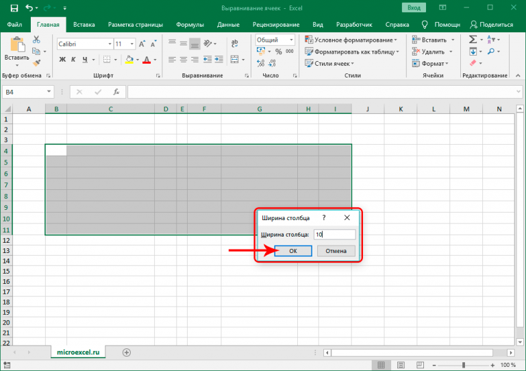
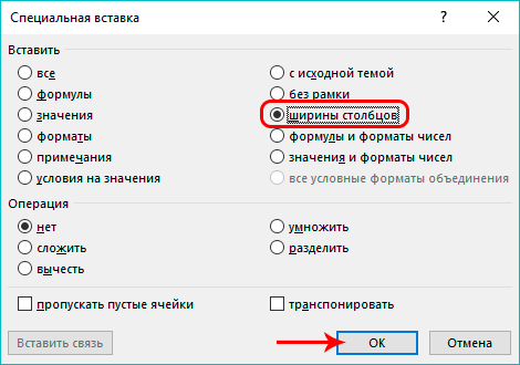
3. Then a dialog box pops up, you need to find a group "ໃສ່"where the item is “Column Width”, and click on the radio button next to it. After selecting it, you can confirm your actions by pressing "ຕົກ​ລົງ".
   

   

4. Then the cell size parameters are changed so that their value is similar to that in the original table.
   

   

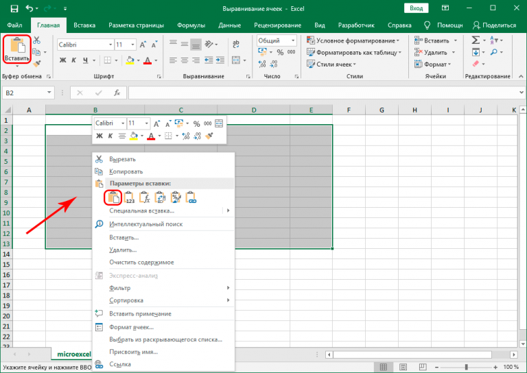
5. That’s it, now it is possible to paste this range into another document or sheet so that the size of its cells matches the original document. This result can be achieved in several ways. You can right-click on the cell that will be the first cell of the table – the one that was copied from another source. Then a context menu will appear, and there you need to find the item "ໃສ່". There is a similar button on the tab "ບ້ານ". But the easiest way is to press the key combination Ctrl + V. Although it is more difficult to remember than using the previous two methods, but when it is memorized, you can save a lot of time.
   

   

It is highly recommended to learn the most common Excel hotkey commands. Every single second of work is not only additional time saved, but also the opportunity to be less tired.

That’s it, now the cell sizes of the two tables will be the same.

Using a Macro to Edit Width and Height

If you often have to make sure that the width and height of the cells are the same, it’s better to write a small macro. To do this, you need to edit the property values ​​using the VBA language. RowHeight и ColumnWidth.

If we talk about theory, then to edit the height and width of the cell, you need to control these row and column parameters.

The macro allows you to adjust the height only in points, and the width in characters. It is not possible to set the units of measure that you need.

To adjust the line height, use the property RowHeight ຈຸດ​ປະ​ສົງ -. For example, yes.

ActiveCell.RowHeight = 10

Here, the height of the row where the active cell is located will be 10 points. 

If you enter such a line in the macro editor, the height of the third line will change, which in our case will be 30 points.

Rows(3).RowHeight = 30

According to our topic, this is how you can change the height of all cells included in a certain range:

Range(«A1:D6»).RowHeight = 20

And like this – the whole column:

Columns(5).RowHeight = 15

The number of the column is given in parentheses. It is the same with strings – the number of the string is given in brackets, which is equivalent to the letter of the alphabet corresponding to the number.

To edit the column width, use the property ColumnWidth ຈຸດ​ປະ​ສົງ -. The syntax is similar. That is, in our case, you need to decide on the range that you want to change. Let it be A1:D6. And then write the following line of code:

Range(«A1:D6»).ColumnWidth = 25

As a consequence, each cell within this range is 25 characters wide.

Which method to choose?

First of all, you need to focus on the tasks that the user needs to complete. In general, it is possible to adjust the width and height of any cell using manual adjustments down to the pixel. This method is convenient in that it is possible to adjust the exact width-to-height ratio of each of the cells. The disadvantage is that it takes more time. After all, you must first move the mouse cursor over the ribbon, then enter the height separately from the keyboard, separately the width, press the “OK” button. All this takes time.

In turn, the second method with manual adjustment directly from the coordinate panel is much more convenient. You can literally in two mouse clicks make the correct size settings for all cells of a sheet or a specific fragment of a document.

A macro, on the other hand, is a fully automated option that allows you to edit cell parameters in just a few clicks. But it requires programming skills, although it is not so difficult to master it when it comes to simple programs.

ບົດສະຫຼຸບ

Thus, there are several different methods for adjusting the width and height of cells, each of which is suitable for certain tasks. As a result, the table can become very pleasant to look at and comfortable to read. Actually, all this is done for this. Summarizing the information obtained, we obtain the following methods:

1. Editing the width and height of a specific range of cells through a group "ຈຸລັງ", ຊຶ່ງສາມາດພົບເຫັນຢູ່ໃນແຖບ "ບ້ານ".
2. Editing cell parameters of the entire document. To do this, you must click on the combination Ctrl + A or on a cell at the junction of a column with line numbers and a line with alphabetic column names.
3. Manual adjustment of cell sizes using the coordinate panel. 
4. Automatic adjustment of cell sizes so that they fit the copied fragment. Here they are made the same size as the table that was copied from another sheet or workbook.

In general, there is nothing complicated about this. All the described methods are understandable on an intuitive level. It is enough to apply them several times in order to be able not only to use them yourself, but also to teach someone the same.